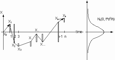
The Wiener process assumes a step size d which could be a step back or forth with equal probability 1/2.

The parameter h denotes the time increment. a determines the ratio between d ²/h when both go to zero. The rational for this specific definition will be given below. We are now looking for the distribution of D X.

D X will approach a gaussian distribution with zero mean and variance t*d ²/h when we reduce the step size and the time increment at the same time leading to an infinite number of steps

f(D X_t) ~ N(0,t*d ²/h)

according to the central limit the theorem.

d ²/h could disappear when both the step size and the time increment go to zero at the same pace. This would describe a situation without any motion. The other extreme would be that d ²/h grows over all limits when h goes faster to zero. This is also not leads to an interesting system.

The remaining possibility is that d and h approach zero in such a way that d ²/h becomes a constant a because both do not depend on t which lead to the below definition for the step size.

It is important to note that the variance t*d ²/h can grow over all limits proportional to time t. D X_t is called Wiener process W(t) or Brownian motion B(t). The Wiener process D X_t is not a stationary process.

W(t) could also be conceived the Wiener process as the integral of the white noise process S(t)

with the spectral density a and the distribution f_s(s) ~ N(0, t*a ). a is also known as diffusion coefficient.

Finally, we can describe the Wiener process also by a stochastic differential equation when introducing a differential notation dW(t):

W_S denotes the standard Wiener process with variance equal one. Whereby the following equation holds true for the expectation value of dWs:

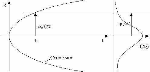
The probability density function is the gaussian distribution with zero mean value and a time variation.

The diagram demonstrates how the gaussian distribution expands over time where the expanding standard deviation is proportional to the square root of time. This means that the probability distribution is different at each point in time.